opinf.ddt

Tools for estimating snapshot time derivatives.

Classes

DerivativeEstimatorTemplate	Template for time derivative estimators.
UniformFiniteDifferencer	Time derivative estimation with finite differences for state snapshots spaced uniformly in time.
NonuniformFiniteDifferencer	Time derivative estimation with finite differences for state snapshots that are not spaced uniformly in time.
InterpDerivativeEstimator	Time derivative estimator based on interpolation.

Finite Difference Schemes for Uniformly Spaced Data

Forward Differences

fwd1	First-order forward difference for estimating the first derivative.
fwd2	Second-order forward difference for estimating the first derivative.
fwd3	Third-order forward difference for estimating the first derivative.
fwd4	Fourth-order forward difference for estimating the first derivative.
fwd5	Fifth-order forward difference for estimating the first derivative.
fwd6	Sixth-order forward difference for estimating the first derivative.

Backward Differences

bwd1	First-order backward difference for estimating the first derivative.
bwd2	Second-order backward difference for estimating the first derivative.
bwd3	Third-order backward difference for estimating the first derivative.
bwd4	Fourth-order backward difference for estimating the first derivative.
bwd5	Fifth-order backward difference for estimating the first derivative.
bwd6	Sixth-order backward difference for estimating the first derivative.

Central Differences

ctr2	Second-order central difference for estimating the first derivative.
ctr4	Fourth-order central difference for estimating the first derivative.
ctr6	Sixth-order central difference for estimating the first derivative.

Mixed Differences

ord2	Second-order forward, central, and backward differences for estimating the first derivative.
ord4	Fourth-order forward, central, and backward differences for estimating the first derivative.
ord6	Sixth-order forward, central, and backward differences for estimating the first derivative.
ddt_uniform	Forward, central, and backward differences for estimating the first derivative.

Finite Difference Schemes for Nonuniformly Spaced Data

ddt_nonuniform	Second-order finite differences for estimating the first derivative.
ddt	Finite differences for estimating the first derivative.

Overview

• Operator Inference for continuous models requires time derivatives of the state snapshots.

• opinf.ddt provides tools for estimating the time derivatives of the state snapshots.

• Finite difference approximations are available through UniformFiniteDifferencer and NonuniformFiniteDifferencer.

import opinf
import numpy as np
import scipy.interpolate as spinterpolate

opinf.utils.mpl_config()

Time Derivative Estimation

To calibrate time-continuous models, Operator Inference requires the time derivative of the state snapshots. For example, consider the LTI system

(10)\[ \begin{aligned} \ddt\qhat(t) = \Ahat\qhat(t) + \Bhat\u(t). \end{aligned} \]

Here, \(\qhat(t)\in\RR^{r}\) is the time-dependent (reduced-order) state and \(\u(t)\in\RR^{m}\) is the time-dependent input. In order to learn \(\Ahat\) and \(\Bhat\), Operator Inference solves a regression problem of the form

\[ \begin{aligned} \min_{\Ahat,\Bhat}\sum_{j=0}^{k-1}\left\| \Ahat\qhat_j + \Bhat\u_j - \dot{\qhat}_j \right\|_2^2 \end{aligned} \]

or similar, where each triplet \((\qhat_j, \dot{\qhat}_j, \u_j)\) should correspond to the solution of (10) at some time \(t_j\), \(j = 0, \ldots, k - 1\). In particular, we want

\[ \begin{aligned} \dot{\qhat}_j \approx \ddt\qhat(t)\big|_{t = t_j} = \Ahat\qhat_j + \Bhat\u_j. \end{aligned} \]

This module provides tools for estimating the snapshot time derivatives \(\dot{\qhat}_0,\ldots,\dot{\qhat}_{k-1}\in\RR^{r}\) from the reduced snapshots \(\qhat_0,\ldots,\qhat_{k-1}\in\RR^{r}\).

Preprocessing and Time Derivatives

In some cases, a full-order model may provide snapshot time derivatives \(\dot{\q}_0,\ldots,\dot{\q}_{k-1}\in\RR^{n}\) in addition to state snapshots \(\q_0,\ldots,\q_{k-1}\in\RR^{n}\). If any lifting or preprocessing steps are used on the state snapshots, be careful to use the appropriate transformation for snapshot time derivatives, which may be different than the transformation used on the snapshots themselves.

For example, consider the affine state approximation \(\q(t) \approx \Vr\qhat(t) + \bar{\q}\) with an orthonormal basis matrix \(\Vr\in\RR^{n\times r}\) and a fixed vector \(\bar{\q}\in\RR^{n}\). In this case,

\[ \begin{aligned} \ddt\q(t) \approx \ddt\left[\Vr\qhat(t) + \bar{\q}\right] = \Vr\ddt\left[\qhat(t)\right]. \end{aligned} \]

Hence, while the compressed state snapshots are given by \(\qhat_j = \Vr\trp(\q_j - \bar{\q})\), the correct compressed snapshot time derivatives are \(\dot{\qhat}_j = \Vr\trp\dot{\q}_j\) (without the \(\bar{\q}\) shift).

See opinf.lift.LifterTemplate.lift_ddts() and opinf.pre.TransformerTemplate.transform_ddts().

Finite Difference Estimators

Partial Estimation

Every finite difference scheme has limitations on where the derivative can be estimated. For example, a first-order backward scheme requires \(\qhat(t_{j-1})\) and \(\qhat(t_j)\) to estimate \(\dot{\qhat}(t_j)\), hence the derivative cannot be estimated at \(t = t_0\).

The forward, backward, and central difference functions (fwd1(), bwd3(), ctr6(), etc.) take in a snapshot matrix \(\Qhat\in\RR^{r\times k}\), a time step, and (optionally) the corresponding input matrix \(\U\in\RR^{m\times k}\) and return a subset of the snapshots \(\Qhat'\in\mathbb{R}^{r\times k'}\), the corresponding derivatives \(\dot{\Qhat}\in\RR^{r\times k'}\), and (optionally) the corresponding inputs \(\U'\in\RR^{m \times k'}\).

# Set a state dimension, input dimension, and number of snapshots.
r = 20
m = 3
k = 400

# Make test data.
t = np.linspace(0, 1, k)
Q = np.random.random((r, k))
U = np.random.random((m, k))

# Extract the time step.
dt = t[1] - t[0]

Qnew, Qdot = opinf.ddt.bwd2(states=Q, dt=dt)
print(f"{Qnew.shape=}, {Qdot.shape=}")

Qnew.shape=(20, 398), Qdot.shape=(20, 398)

Qnew, Qdot, Unew = opinf.ddt.ctr6(states=Q, dt=dt, inputs=U)
print(f"{Qnew.shape=}, {Qdot.shape=}, {Unew.shape=}")

Qnew.shape=(20, 394), Qdot.shape=(20, 394), Unew.shape=(3, 394)

Complete Estimation

The finite difference functions ord2(), ord4(), and ord6() mix forward, central, and backward differences to provide derivative estimates for all provided state snapshots. These schemes are used by ddt_uniform(), and ddt_nonuniform(), which only return the estimated derivatives.

Qnew, Qdot = opinf.ddt.ord4(states=Q, dt=dt)
print(f"{Qnew.shape=}, {Qdot.shape=}")
print(f"{(Qnew is Q)=}")

Qnew.shape=(20, 400), Qdot.shape=(20, 400)
(Qnew is Q)=True

Qdot = opinf.ddt.ddt_uniform(states=Q, dt=dt, order=4)
print(f"{Qdot.shape=}")

Qdot.shape=(20, 400)

Qdot = opinf.ddt.ddt_nonuniform(states=Q, t=t)
print(f"{Qdot.shape=}")

Qdot.shape=(20, 400)

Convenience Classes

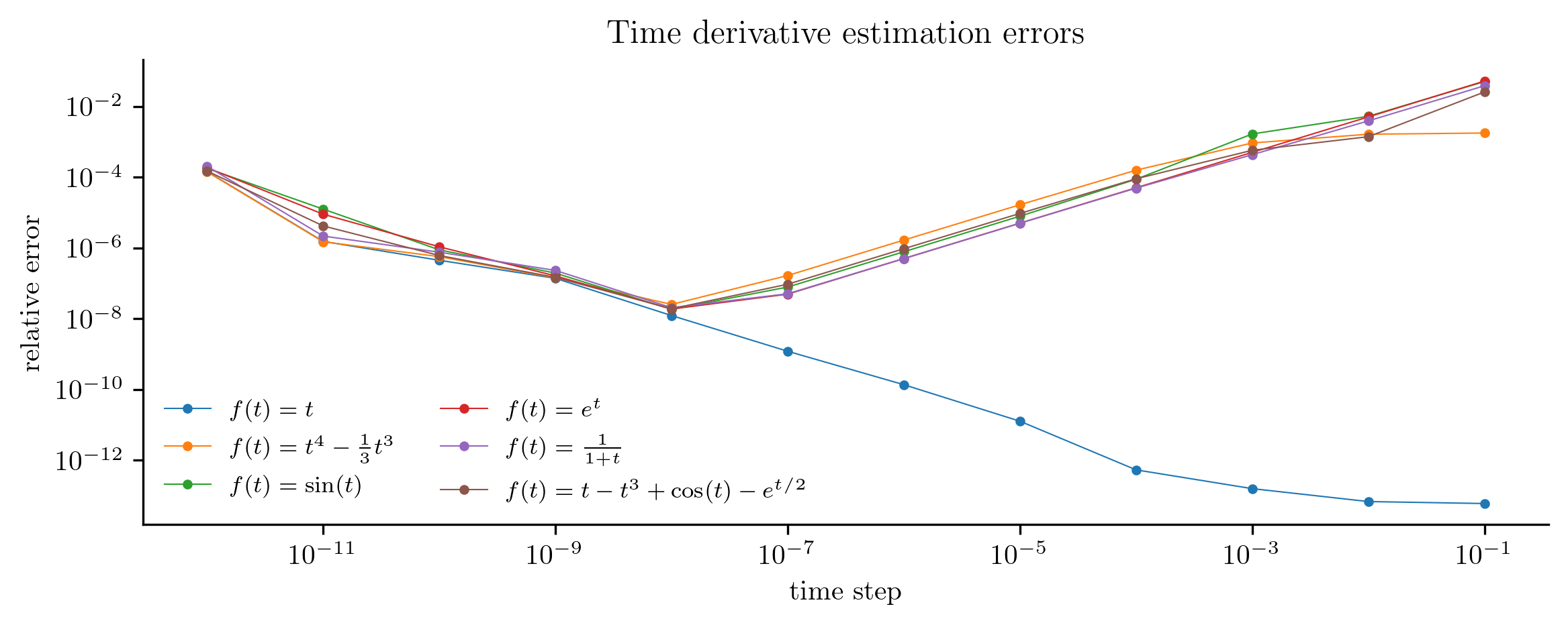
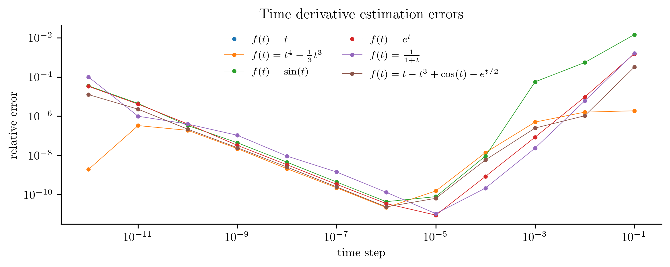
The classes UniformFiniteDifferencer and NonuniformFiniteDifferencer wrap the finite difference methods listed above for use with opinf.roms classes. They also have a verify() method for checking the estimation scheme against true derivatives for a limited set of test cases.

differ = opinf.ddt.UniformFiniteDifferencer(t, scheme="fwd1")
print(differ)

UniformFiniteDifferencer
  time_domain: 400 entries in [0.0, 1.0]
  dt:          2.5063e-03
  scheme:      fwd1()

differ.verify(plot=True)

estimate() output shapes are consistent

Qnew, Qdot, Unew = differ.estimate(states=Q, inputs=U)
print(f"{Qnew.shape=}, {Qdot.shape=}, {Unew.shape=}")

Qnew.shape=(20, 399), Qdot.shape=(20, 399), Unew.shape=(3, 399)

Interpolatory Estimators

The InterpDerivativeEstimator interpolates the state data using classes from scipy.interpolate and evaluates the derivative of the interpolant.

estimator = opinf.ddt.InterpDerivativeEstimator(t, "pchip")
print(estimator)

InterpDerivativeEstimator
  time_domain: 400 entries in [0.0, 1.0]
  InterpolatorClass: PchipInterpolator()

estimator.verify(plot=True)

estimate() output shapes are consistent

Custom Estimators

New time derivative estimators can be defined by inheriting from DerivativeEstimatorTemplate. Once implemented, the verify() method may be used to compare the results of estimate() with true derivatives for a limited number of test cases.

class MyEstimator(opinf.ddt.DerivativeEstimatorTemplate):
    """Inheritance template for custom derivative estimators."""

    # Constructor -------------------------------------------------------------
    def __init__(self, time_domain, hyperparameters):
        """Set any hyperparameters.
        If there are no hyperparameters, __init__() may be omitted.
        """
        super().__init__(time_domain)
        # Process hyperparameters here.

    # Required methods --------------------------------------------------------
    def estimate(self, states, inputs=None):
        """Estimate the first time derivatives of the states.

        Parameters
        ----------
        states : (r, k) ndarray
            State snapshots, either full or (preferably) reduced.
        inputs : (m, k) ndarray or None
            Inputs corresponding to the state snapshots, if applicable.

        Returns
        -------
        _states : (r, k') ndarray
            Subset of the state snapshots.
        ddts : (r, k') ndarray
            First time derivatives corresponding to ``_states``.
        _inputs : (m, k') ndarray or None
            Inputs corresponding to ``_states``, if applicable.
            **Only returned** if ``inputs`` is provided.
        """
        raise NotImplementedError

Example: Cubic Spline Interpolation

The following class wraps scipy.interpolate.CubicSpline and uses its derivative() method to compute the derivative. This is a simplified version of DerivativeEstimatorTemplate.

class CubicSplineEstimator(opinf.ddt.DerivativeEstimatorTemplate):
    """Derivative estimator using cubic spline interpolation."""

    # Constructor -------------------------------------------------------------
    def __init__(self, time_domain, bc_type="not-a-knot"):
        """Save arguments for scipy.interpolate.CubicSpline."""
        super().__init__(time_domain)
        self.options = dict(bc_type=bc_type, axis=1, extrapolate=None)

    # Required methods --------------------------------------------------------
    def estimate(self, states, inputs=None):
        """Estimate the first time derivatives of the states."""
        spline = spinterpolate.CubicSpline(
            x=self.time_domain,
            y=states,
            **self.options,
        )
        ddts = spline(self.time_domain, 1)
        if inputs is None:
            return states, ddts
        return states, ddts, inputs

spline_estimator = CubicSplineEstimator(t)
print(spline_estimator)

CubicSplineEstimator
  time_domain: 400 entries in [0.0, 1.0]

spline_estimator.verify()

estimate() output shapes are consistent

Time derivative estimation relative errors
===========================================

f(t) = t
--------
dt = 1.0e-01:	error = 4.5211e-17
dt = 1.0e-02:	error = 5.0120e-17
dt = 1.0e-03:	error = 1.8298e-16
dt = 1.0e-04:	error = 0.0000e+00
dt = 1.0e-05:	error = 3.6467e-17
dt = 1.0e-06:	error = 1.8057e-16
dt = 1.0e-07:	error = 5.1811e-17
dt = 1.0e-08:	error = 9.7815e-17
dt = 1.0e-09:	error = 8.7375e-17
dt = 1.0e-10:	error = 8.1770e-17
dt = 1.0e-11:	error = 1.8568e-17
dt = 1.0e-12:	error = 2.1054e-17

f(t) = t^4 - \frac{1}{3}t^3
---------------------------
dt = 1.0e-01:	error = 1.2794e-10
dt = 1.0e-02:	error = 9.7208e-11
dt = 1.0e-03:	error = 1.3701e-11
dt = 1.0e-04:	error = 3.1429e-13
dt = 1.0e-05:	error = 3.4617e-12
dt = 1.0e-06:	error = 3.7101e-11
dt = 1.0e-07:	error = 3.6571e-10
dt = 1.0e-08:	error = 3.5725e-09
dt = 1.0e-09:	error = 3.6626e-08
dt = 1.0e-10:	error = 3.0326e-07
dt = 1.0e-11:	error = 4.3497e-07
dt = 1.0e-12:	error = 1.9250e-09

f(t) = \sin(t)
--------------
dt = 1.0e-01:	error = 8.0269e-06
dt = 1.0e-02:	error = 1.1179e-08
dt = 1.0e-03:	error = 2.5254e-11
dt = 1.0e-04:	error = 7.6142e-13
dt = 1.0e-05:	error = 7.7015e-12
dt = 1.0e-06:	error = 7.0952e-11
dt = 1.0e-07:	error = 7.4745e-10
dt = 1.0e-08:	error = 7.5327e-09
dt = 1.0e-09:	error = 7.2757e-08
dt = 1.0e-10:	error = 5.3670e-07
dt = 1.0e-11:	error = 6.4461e-06
dt = 1.0e-12:	error = 5.6887e-05

f(t) = e^t
----------
dt = 1.0e-01:	error = 7.1984e-05
dt = 1.0e-02:	error = 2.5971e-08
dt = 1.0e-03:	error = 9.5341e-12
dt = 1.0e-04:	error = 5.2738e-13
dt = 1.0e-05:	error = 5.5413e-12
dt = 1.0e-06:	error = 5.8298e-11
dt = 1.0e-07:	error = 5.4748e-10
dt = 1.0e-08:	error = 5.5524e-09
dt = 1.0e-09:	error = 5.4111e-08
dt = 1.0e-10:	error = 6.5194e-07
dt = 1.0e-11:	error = 6.6393e-06
dt = 1.0e-12:	error = 5.9876e-05

f(t) = \frac{1}{1 + t}
----------------------
dt = 1.0e-01:	error = 1.6470e-04
dt = 1.0e-02:	error = 6.6734e-08
dt = 1.0e-03:	error = 2.5902e-11
dt = 1.0e-04:	error = 2.5069e-12
dt = 1.0e-05:	error = 2.1458e-11
dt = 1.0e-06:	error = 1.7157e-10
dt = 1.0e-07:	error = 2.6194e-09
dt = 1.0e-08:	error = 1.2829e-08
dt = 1.0e-09:	error = 1.4667e-07
dt = 1.0e-10:	error = 5.1856e-07
dt = 1.0e-11:	error = 1.3063e-06
dt = 1.0e-12:	error = 1.2844e-04

f(t) = t - t^3 + \cos(t) - e^{t/2}
----------------------------------
dt = 1.0e-01:	error = 6.8445e-06
dt = 1.0e-02:	error = 4.3418e-10
dt = 1.0e-03:	error = 5.1397e-13
dt = 1.0e-04:	error = 3.7421e-13
dt = 1.0e-05:	error = 4.1815e-12
dt = 1.0e-06:	error = 3.9533e-11
dt = 1.0e-07:	error = 4.1749e-10
dt = 1.0e-08:	error = 4.1424e-09
dt = 1.0e-09:	error = 4.1958e-08
dt = 1.0e-10:	error = 3.1348e-07
dt = 1.0e-11:	error = 3.4228e-06
dt = 1.0e-12:	error = 2.3170e-05