opinf.basis#
Tools for compressing state data.
Classes
Template class for bases. |
|
Join bases together for states with multiple variables. |
|
Linear low-dimensional state approximation. |
|
Proper othogonal decomposition basis, consisting of the principal left singular vectors of a collection of states. |
Functions
Compute a POD basis from the given states. |
|
Use the method of snapshots to compute the left singular values of a collection of state snapshots. |
|
Compute the number of singular values needed to surpass a given cumulative energy threshold. |
|
Compute the number of singular values needed such that the residual energy drops beneath a given threshold. |
|
Count the number of normalized singular values that are greater than a specified threshold. |
Overview
opinf.basisclasses define mappings between high-dimensional states and low-dimensional latent coordinates.The most common low-dimensional state approximation for Operator Inference is Proper Orthogonal Decomposition.
Multivariable data can be treated jointly (monolithic) or variable by variable (multilithic).
Example Data
Some examples on this page use data from a compressible flow problem for an ideal gas as described in [GMW22, QKPW20].
State Variables
The data consists of three variables recorded at \(k = 200\) points in time:
Velocity \(v\),
Pressure \(p\), and
Specific volume (inverse density) \(\xi = 1/\rho\).
The spatial discretization results in \(400\) degrees of freedom per variable, i.e., \(n = 3 \times 400 = 1{,}200\).
You can download the data here to repeat the demonstration.
import warnings
import numpy as np
import scipy.linalg as la
import matplotlib.pyplot as plt

import opinf

# Suppress some warning printouts.
warnings.showwarning = lambda msg, cat, *args: print(f"{cat.__name__}: {msg}")
opinf.utils.mpl_config()
Low-dimensional Approximations#
Reduced-order models enact a computational speedup by approximating the \(n\)-dimensional system state with \(r \ll n\) degrees of freedom and working in the reduced state space.
The opinf.basis module provides tools for constructing low-dimensional state approximations.
Notation
On this page,
\(\q \in \RR^n\) denotes the high-dimensional state vector to be reduced (the full state),
\(\qhat\in\RR^r\) is the low-dimensional, compressed version of \(\q\) (the reduced state),
\(\breve{\q}\in\RR^n\) is the high-dimensional, decompressed version of \(\qhat\) (the reconstructed state),
\(\boldsymbol{\Gamma}:\RR^r\to\RR^n\) is the decompression function defining the approximation of \(\q\) with \(\qhat\) (sometimes called the decoder), and
\(\boldsymbol{\Gamma}^{*}:\RR^n\to\RR^r\) is the compression function corresponding to \(\boldsymbol{\Gamma}\) (sometimes called the encoder).
That is, \(\qhat = \boldsymbol{\Gamma}^{*}(\q)\) and \(\q \approx \breve{\q} = \boldsymbol{\Gamma}(\qhat)\).

We assume that the full state \(\q\) has already been preprocessed, for instance with the tools described in opinf.pre.
For a given \(\boldsymbol{\Gamma}\) and norm \(\|\cdot\|\), the natural compression function \(\boldsymbol{\Gamma}^{*}\) is the one that minimizes the approximation error induced by \(\boldsymbol{\Gamma}\):
In this case, \(P = \boldsymbol{\Gamma} \circ \boldsymbol{\Gamma}^{*}:\RR^n\to\RR^n\) satisfies \(P(P(\q)) = P(\q)\) for all \(\q\in\RR^{n}\) and \(P\) is called a projection. The error between \(\breve{\q} = P(\q)\) and \(\q\) is called the projection error at \(\q\), and \(\breve{\q}\) is, by definition, the closest point to \(\q\) in \(\operatorname{range}(\boldsymbol{\Gamma})\).
Proof
For any \(\tilde{\q}\in\RR^r\), we have
By inspection, setting \(\qhat = \tilde{\q}\) achieves the minimal value of zero. Hence, \(\boldsymbol{\Gamma}^{*}(\boldsymbol{\Gamma}(\tilde{\q})) = \tilde{\q}\), and we have
Basis API
opinf.basis classes are equipped with the following methods.
fit()uses state data to learn appropriate decompression / compression functions.compress()applies the compression function \(\boldsymbol{\Gamma}^{*}\).decompress()applies the decompression function \(\boldsymbol{\Gamma}\).project()applies the composition \(\boldsymbol{\Gamma}\circ\boldsymbol{\Gamma}^{*}\).projection_error()computes the relative or absolute error of the projection at a given state.verify()checks that composingdecompress()withcompress()defines a projection.
Linear Bases#
A linear basis approximates approximates the full state \(\q\in\RR^n\) as a linear combination of \(r\) basis vectors \(\v_1,\ldots,\v_r\in\RR^n\). Mathematically, this means the reconstructed state \(\breve{\q}\in\RR^n\) is contained in the \(r\)-dimensional linear subspace \(\operatorname{span}(\{\v_1,\ldots,\v_r\})\subset\RR^n\). The reduced state vector \(\qhat = [~\hat{q}_1~~\cdots~~\hat{q}_r~]\trp\in\RR^r\) consists of latent coordinate coefficients for each basis vector.
Gathering the basis vectors into the basis matrix \(\Vr = [~\v_1~~\cdots~~\v_r~]\in\RR^{n\times r}\), a linear basis approximation is given by
If the basis vectors are orthonormal, i.e., \(\Vr\trp\Vr = \I\in\RR^{r\times r}\), then the compression function is defined by the application of \(\Vr\trp\).
Compression
\(\boldsymbol{\Gamma}^{*} : \q \mapsto \Vr\trp\q\)
Decompression
\(\boldsymbol{\Gamma} : \qhat \mapsto \Vr\qhat\)
Projection
\(\boldsymbol{\Gamma}\circ\boldsymbol{\Gamma}^{*} : \q \mapsto \Vr\Vr\trp\q\).
Derivation of \(~\boldsymbol{\Gamma}^{*}\)
As stated above, the optimal compression function is defined by
This is a linear least-squares problem; the solution is given by the normal equations
which simplifies to \(\qhat = \Vr\trp\q\) since \(\Vr\trp\Vr = \I\).
In general, \(\qhat = (\Vr\trp\Vr)^{-1}\Vr\q = \Vr^{\dagger}\q\), where \(\Vr^{\dagger}\) is the Moore–Penrose pseudoinverse of \(\Vr\).
Known Basis Matrix#
The LinearBasis class creates a linear basis from a given, orthonormal basis matrix.
Unlike the other classes in this module, LinearBasis.compress() and LinearBasis.decompress() can be used immediately after instantiation because the basis matrix is provided up front instead of learned from state data in LinearBasis.fit().
The basis matrix is accessible via the entries attribute or by indexing with [:].
Non-orthonormal Bases
LinearBasis raises a warning if initialized with a basis matrix \(\Vr\) whose columns are not orthonormal.
To avoid this issue, a basis matrix can be orthonormalized (without changing the column span) through the Gram–Schmidt process via, e.g., scpiy.linalg.qr().
>>> import scipy.linalg as la

>>> Vr_orth = la.qr(Vr, mode="economic")[0]
The following code uses a LinearBasis for a trigonometric basis representing the functions \(\sin(2\pi x)\), \(\sin(4\pi x)\), …, \(\sin(2r\pi x)\) evaluated over a one-dimensional spatial domain.
# Choose full and reduced state dimensions.
n = 500
r = 8

# Define a spatial domain and evaluate the basis functions over that domain.
x = np.linspace(0, 1, n)
Vr = np.column_stack([np.sin(2 * k * np.pi * x) for k in range(1, r + 1)])

# Check to see if Vr has orthonormal columns.
np.round(Vr.T @ Vr, 4)
array([[249.5,   0. ,  -0. ,   0. ,  -0. ,  -0. ,  -0. ,  -0. ],
       [  0. , 249.5,   0. ,   0. ,   0. ,   0. ,  -0. ,   0. ],
       [ -0. ,   0. , 249.5,  -0. ,  -0. ,  -0. ,   0. ,   0. ],
       [  0. ,   0. ,  -0. , 249.5,  -0. ,   0. ,   0. ,   0. ],
       [ -0. ,   0. ,  -0. ,  -0. , 249.5,   0. ,  -0. ,   0. ],
       [ -0. ,   0. ,  -0. ,   0. ,   0. , 249.5,   0. ,  -0. ],
       [ -0. ,  -0. ,   0. ,   0. ,  -0. ,   0. , 249.5,   0. ],
       [ -0. ,   0. ,   0. ,   0. ,   0. ,  -0. ,   0. , 249.5]])
Because \(\Vr\trp\Vr\) is diagonal but not the identify matrix, these basis vectors are orthogonal but do not have unit length.
Using this basis matrix to initialize a LinearBasis results in a warning; additionally, calling LinearBasis.verify() raises an error ot indicate that composing the decompression and compression functions does not define a projection.
trig_basis = opinf.basis.LinearBasis(Vr)

try:
    trig_basis.verify()
except Exception as ex:
    print(f"{type(ex).__name__}: {ex}")
OpInfWarning: basis not orthogonal
VerificationError: project(project(states)) != project(states)
To normalize the basis matrix, we divide each column vector by its norm.
# Normalize the columns of the basis matrix.
Vr_orth = Vr / la.norm(Vr, axis=0)
trig_basis_orth = opinf.basis.LinearBasis(Vr_orth)
# Print dimensions and check that the basis matrix is orthonormal.
print(trig_basis_orth)
trig_basis_orth.verify()
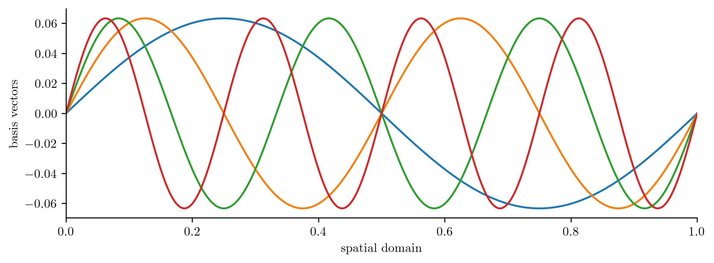
# Plot the first few basis vectors as functions of x.
trig_basis_orth.plot1D(x, num_vectors=4)
plt.show()
LinearBasis
  full_state_dimension:    500
  reduced_state_dimension: 8
compress() and decompress() are consistent
The next code block checks how well the function \(f(x) = x(1 - x)e^x\) can be approximated by this basis.
# Represent a new function in the span of the basis.
f = x * (1 - x) * np.exp(x)
f_projected = trig_basis_orth.project(f)

# Compute the projection error for the new function.
error = trig_basis_orth.projection_error(f)
print(f"Relative projection error: {error:%}")

# Plot the original function and its projection with this basis.
plt.plot(x, f, label="$f(x)$")
plt.plot(x, f_projected, label="$f(x)$ projected")
plt.legend(loc="upper left")
plt.show()
Relative projection error: 98.274670%
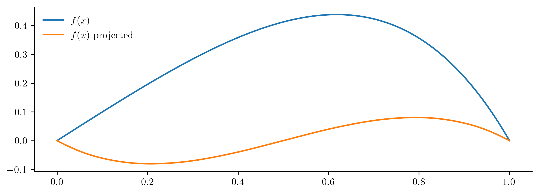
The projection is a poor approximation for the original function because \(f(x)\) lies well outside of the span of the basis functions \(\sin(2\pi x),\ldots,\sin(2r\pi x)\). A better option is a Fourier basis consisting of cosines as well as sines.
# Construct basis vectors with cosines and sines.
Vr_raw = np.column_stack(
    [np.cos(2 * k * np.pi * x) for k in range(r // 2)]
    + [np.sin(2 * k * np.pi * x) for k in range(1, (r // 2) + 1)]
)

# Orthonormalize the basis with the Gram-Schmidt process.
Vr_orth = la.qr(Vr_raw, mode="economic")[0]
fourier_basis = opinf.basis.LinearBasis(Vr_orth)

# Print dimensions and check that the basis matrix is orthonormal.
print(fourier_basis)
fourier_basis.verify()

# Calculate the projection of f(x) and its relative projection error.
f_projected = fourier_basis.project(f)
error = fourier_basis.projection_error(f)
print(f"Relative projection error: {error:%}")

# Plot the original function and its projection with this new basis.
plt.plot(x, f, label="$f(x)$")
plt.plot(x, f_projected, label="$f(x)$ projected")
plt.legend(loc="upper left")
plt.show()
LinearBasis
  full_state_dimension:    500
  reduced_state_dimension: 8
compress() and decompress() are consistent
Relative projection error: 3.753152%
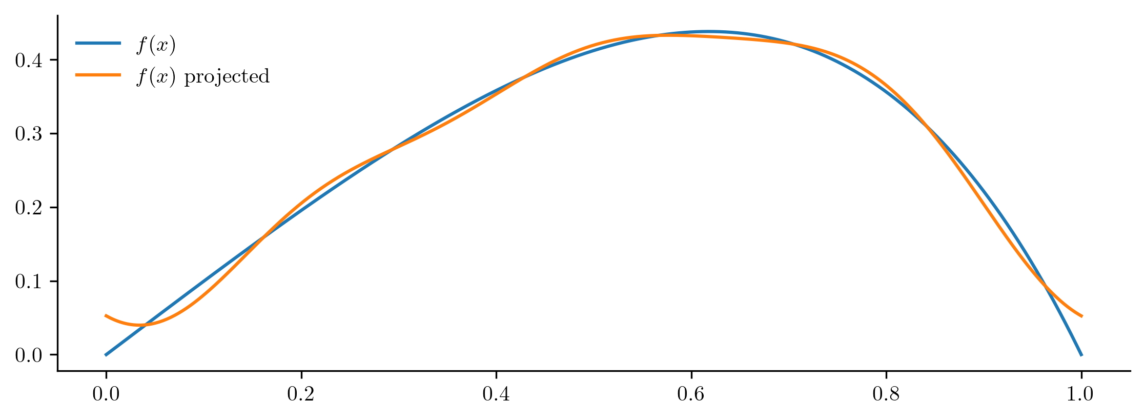
The approximation with the Fourier basis is much better than with the sine basis, even when they have same number of basis vectors. In general, using more basis vectors improves the approximation power of the basis and decreases projection error.
Proper Orthogonal Decomposition#
There is no one basis that works well for every problem.
The PODBasis class uses Proper Orthogonal Decomposition (POD), a close relative of Principal Component Analysis (PCA), to construct a linear basis that is tailored to a provided set of state data.
This is the most common basis used in Operator Inference applications.
Definition#
In finite dimensions, POD is computed by taking the singular value decomposition (SVD) of a snapshot matrix \(\Q = [~\q_0~~\cdots~~\q_{k-1}~]\in\RR^{n\times k}\). If \(\boldsymbol{\Phi\Sigma\Psi}\trp = \Q\) is the SVD, then the rank-\(r\) POD basis is \(\Vr = \boldsymbol{\Phi}_{:,:r}\), the matrix comprising the first \(r\) left singular vectors. Since the singular vectors are orthogonal, we always have \(\Vr\trp\Vr = \I\).
# Load the example snapshot data.
snapshots = np.load("basis_example.npy")
snapshots.shape
---------------------------------------------------------------------------
FileNotFoundError                         Traceback (most recent call last)
Cell In[7], line 2
      1 # Load the example snapshot data.
----> 2 snapshots = np.load("basis_example.npy")
      3 snapshots.shape

File ~/Software/OpInf/.tox/docs/lib/python3.13/site-packages/numpy/lib/_npyio_impl.py:454, in load(file, mmap_mode, allow_pickle, fix_imports, encoding, max_header_size)
    452     own_fid = False
    453 else:
--> 454     fid = stack.enter_context(open(os.fspath(file), "rb"))
    455     own_fid = True
    457 # Code to distinguish from NumPy binary files and pickles.

FileNotFoundError: [Errno 2] No such file or directory: 'basis_example.npy'
# Extract the pressure variable from the snapshot data.
velocity, pressure, sp_volume = np.split(snapshots, 3, axis=0)

pressure.shape
# Construct a POD basis with a specified number of basis vectors.
r = 6
pressure_basis = opinf.basis.PODBasis(num_vectors=r, name="pressure")
pressure_basis.fit(pressure)
print(pressure_basis)

# Plot the first few vectors.
pressure_basis.plot1D()
plt.show()
Selecting the Reduced Dimension#
By default, PODBasis.fit() stores all computed basis vectors, and the reduced state dimension \(r\) can be changed on the fly with PODBasis.set_dimension().
In this case, we can increase the reduced state dimension up to \(k = 200\).
However, we often don’t need (or want) all \(k\) basis vectors—as \(r\) increases so does the computational cost of solving the eventual reduced-order model, and at some point adding additional vectors does not significantly increase the approximation power of the basis.
The singular values of the snapshot matrix \(\Q\) can provide guidance for choosing an appropriate reduced state dimension.
There are four related criteria stemming from the singular values \(\sigma_1 > \sigma_2 > \cdots > \sigma_k\).
PODBasis has methods for visualizing each criteria, and PODBasis.set_dimension() has arguments related to each.
Criterion |
Definition |
|
Visualization |
|---|---|---|---|
Singular value decay |
\(\sigma_i \ge \xi\) for \(i\le r\) |
|
|
Cumulative energy |
\(\frac{\sum_{i=1}^r\sigma_i^2}{\sum_{j=1}^k\sigma_j^2} \ge \kappa\) |
|
|
Residual energy |
\(\frac{\sum_{i=r+1}^k\sigma_i^2}{\sum_{j=1}^k\sigma_j^2} \le \epsilon\) |
|
|
Projection error |
\(\frac{\|\Q - \Vr\Vr\trp\Q\|_F}{\|\Q\|_F} \le \rho\) |
|
These singular value-based selection criteria are all related. In particular, the squared projection error of the snapshot matrix is equal to the residual energy:
Proof
Let \(\Q = \boldsymbol{\Phi}\boldsymbol{\Sigma}\boldsymbol{\Psi}\trp\) be the thin singular value decomposition of \(\Q\in\RR^{n \times k}\), meaning \(\boldsymbol{\Phi}\in\RR^{n\times \ell}\), \(\boldsymbol{\Sigma}\in\RR^{\ell \times \ell}\), and \(\boldsymbol{\Psi}\in\RR^{k\times \ell}\), with \(\boldsymbol{\Phi}\trp\boldsymbol{\Phi} = \boldsymbol{\Psi}\trp\boldsymbol{\Psi} = \I\). Splitting the decomposition into “first \(r\) modes” and “remaining modes” gives
where
We have defined \(\Vr = \boldsymbol{\Phi}_{r}\). Using \(\Vr\trp\boldsymbol{\Phi}_{r} = \Vr\trp\Vr = \I\) and \(\Vr\trp\boldsymbol{\Phi}_{\perp} = \boldsymbol{\Phi}_{r}\boldsymbol{\Phi}_{\perp} = \mathbf{0}\),
That is, \(\Vr\Vr\trp\Q = \Vr\Vr\trp(\Q_{r} + \Q_{\perp}) = \Q_{r}\). It follows that
Since \(\boldsymbol{\Phi}_{\perp}\) and \(\boldsymbol{\Psi}_{\perp}\) have orthonormal columns,
Putting it all together,
PODBasis.plot_energy() visualizes several criteria together.
# Show the number of normalized singular values above a given threshold.
pressure_basis.plot_svdval_decay(threshold=1e-5)
plt.show()
# Set the reduced state dimension based on a singular value threshold.
pressure_basis.set_dimension(svdval_threshold=1e-5)
print(pressure_basis)

# Plot the singular value decay and the singular value energies.
pressure_basis.plot_energy(right=100)
plt.show()
The pod_basis() function computes a POD basis matrix and the corresponding singular values.
The functions svdval_decay(), cumulative_energy(), and residual_energy() visualize the dimension selection criteria.
Centered POD#
PODBasis uses a linear approximation \(\q\approx\Vr\qhat\) with \(\Vr\) derived from the SVD of a snapshot matrix \(\Q = [~\q_0~~\cdots~~\q_{k-1}~]\in\RR^{n \times k}\).
It is often advantageous to first center the training data columnwise, in which case POD coincides with PCA.
This results in an affine state approximation,
To get this kind of approximation, center the snapshot matrix first with opinf.pre.ShiftScaleTransformer, and remember to “uncenter” the results of decompress().
shifter = opinf.pre.ShiftScaleTransformer(centering=True)
pressure_centered = shifter.fit_transform(pressure)

# Train a centered POD basis and plot the first few basis vectors.
pressure_pca = opinf.basis.PODBasis(num_vectors=r).fit(pressure_centered)

# To project the (uncentered) pressure, transform, project, then untransform.
pressure_projected = shifter.inverse_transform(
    pressure_pca.project(shifter.transform(pressure))
)

# Compute the projection error.
la.norm(pressure - pressure_projected) / la.norm(pressure)
# Plot the first few basis vectors.
pressure_pca.plot1D()
plt.show()
The principal basis vector of the previous, non-centered basis is almost constant when compared to the other basis vectors. By contrast, the new, centered basis does not have any relatively constant basis vectors.
# Check the variance of the first basis vector in the non-centered case.
np.var(pressure_basis.entries[:, 0])
# Check the variance of each basis vector in the centered case.
np.var(pressure_pca.entries, axis=0).min()
Applying a centering can be interpreted more or less as removing the principal component of non-centered data. In other words, the principal component of non-centered data is often comparable to the mean of the data.
Multivariable Data#
For systems where the full state consists of several variables (pressure, velocity, temperature, etc.), there are two ways to approach a dimensionality reduction. In this section we use \(\q^{(i)}\in\RR^{n_i}\) to denote the \(i\)-th of \(n_q\) state variables, \(i = 0, \ldots, n_q - 1\). For instance, \(\q^{(0)}\in\RR^{100}\) could represent the velocity measured at \(n_0 = 100\) spatial points and \(\q^{(1)}\in\RR^{200}\) could be the pressure at \(n_1 = 200\) spatial points. In many application the state variables are all defined on the same spatial grid with \(n_x\) nodes, in which case \(n_0 = \cdots = n_{n_q-1} = n_x\).
Monolithic Reduction#
One option is to reduce all state variables jointly by considering the concatenated state
where \(n = \sum_{i=0}^{n_q - 1} n_i\).
A low-dimensional approximation \(\q \approx \boldsymbol{\Gamma}(\qhat)\) and a corresponding compression function \(\boldsymbol{\Gamma}^{*}\) can be used to define a dimensionality reduction without reference to the sub-dimensions \(n_i\).
With this approach, it is often very important to preprocess the state variables so that their entries are of similar magnitude.
For instance, the following code creates a single PODBasis for velocity, pressure, and specific volume jointly without and preprocessing.
# Define a basis using the raw snapshot data for all three variables.
joint_pod = opinf.basis.PODBasis(
    residual_energy=1e-8,
    name="velocity-pressure-specificvolume",
)
joint_pod.fit(snapshots)

print(joint_pod)

# Plot the basis vectors.
joint_pod.plot1D()
plt.show()
This basis is highly suspicious: the left third of the plot above shows the portion of the basis vectors corresponding to the velocity, the middle third is for the pressure, and the final third is for the specific volume. The pressure basis vector entries have a much stronger magnitude than the entries for the other two variables because the pressure data is of much larger magnitude than the other variables. Furthermore, the relative projection error for the snapshot set as a whole is low, but it varies significantly across the variables.
def projection_error_report(snapshots_projected):
    """Compute the projection error for each state variable separately."""
    velocity_proj, pressure_proj, spvol_proj = np.split(snapshots_projected, 3)

    # Compute projection errors for the physical variables individually.
    v_error = la.norm(velocity_proj - velocity) / la.norm(velocity)
    p_error = la.norm(pressure_proj - pressure) / la.norm(pressure)
    s_error = la.norm(spvol_proj - sp_volume) / la.norm(sp_volume)
    joint_error = la.norm(snapshots_projected - snapshots) / la.norm(snapshots)

    # Report the errors.
    print(f"Relative projection error of velocity:\t\t{v_error:.4%}")
    print(f"Relative projection error of pressure:\t\t{p_error:.4%}")
    print(f"Relative projection error of specific volume:\t{s_error:.4%}")
    print(f"Relative projection error of joint variables:\t{joint_error:.4%}")
projection_error_report(joint_pod.project(snapshots))
To improve the basis, one option is to scale each variables to the range \([0, 1]\) using opinf.pre.TransformerMulti.
# Initialize a different scaling for each physical variable.
euler_transformer = opinf.pre.TransformerMulti(
    [
        opinf.pre.ShiftScaleTransformer(
            scaling="minmax",
            name="velocity",
            verbose=True,
        ),
        opinf.pre.ShiftScaleTransformer(
            scaling="minmax",
            name="pressure",
            verbose=True,
        ),
        opinf.pre.ShiftScaleTransformer(
            scaling="minmax",
            name="specific volume",
            verbose=True,
        ),
    ]
)

# Learn and apply the transformation.
snapshots_scaled = euler_transformer.fit_transform(snapshots)
# Learn a new POD basis from the scaled data.
joint_pod.fit(snapshots_scaled)

print(joint_pod)

# Plot the basis vectors.
joint_pod.plot1D(num_vectors=7)
plt.show()
The transition zones between the three variables are still visible, but now the basis vector entries are all of the same order of magnitude. The projection error across the variables is also much more consistent than before (remember to unscale the projection!).
projection_error_report(
    euler_transformer.inverse_transform(joint_pod.project(snapshots_scaled))
)
Multilithic Reduction#
Instead of reducing multiple variables jointly, it is sometimes advantageous to define different reductions for each variable separately. Mathematically, we define approximations \(\q^{(i)} \approx \boldsymbol{\Gamma}_{i}(\qhat^{(i)})\) for \(\qhat^{(i)}\in\RR^{r_i}\) for each \(i = 0, \ldots, n_q - 1\), each with corresponding compression functions \(\boldsymbol{\Gamma}_{i}^{*}:\RR^{r_i}\to\RR^{n_i}\). The state approximation for the joint state \(\q\) is then
where \(r = \sum_{i=0}^{n_q - 1}r_i\). This type of reduction can be helpful for structure preservation because the vector \(\qhat^{(i)}\) is the latent representation for \(\q^{(i)}\), as opposed to the monolithic case in which each of the entries of \(\qhat\) affect every \(\q^{(0)},\ldots,\q^{(n_q-1)}\).
The BasisMulti class joins individual bases to reduce multiple variables independently.
The bases need not have the same dimensions or even be of the same class.
euler_pod = opinf.basis.BasisMulti(
    [
        opinf.basis.PODBasis(residual_energy=1e-8, name="velocity"),
        opinf.basis.PODBasis(projection_error=1e-2, name="pressure"),
        opinf.basis.PODBasis(num_vectors=10, name="specific volume"),
    ],
)

euler_pod.fit(snapshots)
print(euler_pod)
projection_error_report(euler_pod.project(snapshots))
Note that we are working with the non-scaled data again. Because the variables are treated separately, we can easily adjust the accuracy of the approximation.
# Use more basis vectors for the pressure.
euler_pod[1].set_dimension(projection_error=1e-4)
print(euler_pod[1], end="\n\n")

projection_error_report(euler_pod.project(snapshots))
Block-diagonal Linear Basis
In multilithic reduction, if all of the state approximations are linear, then the overall state approximation is linear with a block-diagonal matrix \(\Vr\). Specifically, if \(\q^{(i)} \approx \Vr^{(i)}\qhat^{(i)}\), then the approximation for the joint state is \(\q \approx \Vr\qhat\) where
Custom Bases#
New bases can be defined by inheriting from BasisTemplate.
Once implemented, the verify() method may be used to test for consistency between the required methods.
class MyBasis(opinf.basis.BasisTemplate):
    """Custom basis for dimension reduction."""

    # Constructor -------------------------------------------------------------
    def __init__(self, hyperparameters, name=None):
        """Set any basis hyperparameters.
        If there are no hyperparameters, __init__() may be omitted.
        """
        super().__init__(name)
        # Process/store 'hyperparameters' here.

    # Required methods --------------------------------------------------------
    def fit(self, states):
        """Construct the basis."""
        # Set the state dimensions.
        self.full_state_dimension = NotImplemented
        self.reduced_state_dimension = NotImplemented

        # Learn the basis from `states` to enable compress() and decompress().
        raise NotImplementedError

    def compress(self, states):
        """Map high-dimensional states to low-dimensional latent
        coordinates.
        """
        raise NotImplementedError

    def decompress(self, states_compressed, locs=None):
        """Map low-dimensional latent coordinates to high-dimensional
        states.
        """
        raise NotImplementedError

    # Optional methods --------------------------------------------------------
    # These may be deleted if not implemented.
    def save(self, savefile, overwrite=False):
        """Save the basis to an HDF5 file."""
        return NotImplemented

    @classmethod
    def load(cls, loadfile):
        """Load a basis from an HDF5 file."""
        return NotImplemented
See BasisTemplate for details on the arguments for each method.
Example: Canonical Projection#
The following custom basis reduces the full state vector \(\q\) by selecting a limited number of entries. This strategy is useful for impementing the discrete empirical interpolation method (DEIM).
class CanonicalBasis(opinf.basis.BasisTemplate):
    """Canonical projection basis."""

    def __init__(self, num_elements, name=None):
        """Set the number of locations to keep when the full state is
        compressed.
        """
        super().__init__(name)
        self.reduced_state_dimension = num_elements
        self.indices = None

    def fit(self, states):
        """Randomly select locations to keep when the full state is
        compressed.
        """
        self.full_state_dimension = states.shape[0]
        self.indices = np.sort(
            np.random.choice(
                self.full_state_dimension,
                size=self.reduced_state_dimension,
                replace=False,
            )
        )
        return self

    def compress(self, states):
        """Extract the selected elements from the full state."""
        if self.indices is None:
            raise AttributeError("indices not set, call fit()")
        return states[self.indices]

    def decompress(self, states_compressed, locs=None):
        """Populate a full state with the extracted elements."""
        if self.indices is None:
            raise AttributeError("indices not set, call fit()")

        shape = self.full_state_dimension
        if states_compressed.ndim == 2:
            shape = (self.full_state_dimension, states_compressed.shape[1])

        states = np.zeros(shape, dtype=states_compressed.dtype)
        states[self.indices] = states_compressed
        return states if locs is None else states[locs]

    def save(self, savefile, overwrite=False):
        """Save the basis to an HDF5 file."""
        with opinf.utils.hdf5_savehandle(savefile, overwrite) as hf:
            hf.create_dataset("r", data=[self.reduced_state_dimension])
            if self.indices is not None:
                hf.create_dataset("n", data=[self.full_state_dimension])
                hf.create_dataset("indices", data=self.indices)

    @classmethod
    def load(cls, loadfile):
        """Load a basis from an HDF5 file."""
        with opinf.utils.hdf5_loadhandle(loadfile) as hf:
            basis = cls(hf["r"][0])
            if "n" in hf:
                basis.full_state_dimension = hf["n"][0]
                basis.indices = hf["indices"][:]
            return basis
canon = CanonicalBasis(4, name="pressure").fit(pressure)

print(canon)
canon.verify()